Asymptotic Annalysis_01

Background

Suppose that we have two algorithms, how can we tell which is better?

• We could implement both algorithms, run them both
  • Expensive and error prone
• Preferably, we should analyze them mathematically
  • Algorithm analysis

Asymptotic Analysis

In general, we will always analyze algorithms with respect to one or more variables Examples with one variable:

• The number of items n currently stored in an array or other data structure
• The number of items expected to be stored in an array or other data structure
• The dimensions of an \(n\times n\) matrix Examples with multiple variables:
• Dealing with n objects stored in m memory locations
• Multiplying a \(k\times m\) and an \(m\times n\) matrix
• Dealing with sparse matrices of size \(n\times n\) with m non-zero entries

Linear and Binary Search

There are other algorithms which are significantly faster as the problem size increases

• This plot shows maximum and average number of comparisons to find an entry in a sorted array of size n
  • Linear search
  • Binary search Given an algorithm:
• We need to be able to describe these values (e.g. the number of comparisons) mathematically
• We need a systematic tool of using the description of the algorithm together with the properties of an associated data structure
• We need to do this in a machine-independent way

Quadratic Growth

Consider the two functions

• \[f(n)=n^2\]
• \[g(n)=n^2-3n+2\]
• Around n=0, they look very different
• Around n=1000, they seem not much different
• The absolute difference is large, for example,
  • \[f(1000)=1,000,000\]
  • \[g(1000)= 997,002\]
• But the relative difference is very small
  • \[\left | \frac{f(1000)-g(1000)}{f(1000)} \right|= 0.002998 < 0.3%\]
• This difference goes to zero as \(n\rightarrow \infty\)
  • \[\lim_{n\rightarrow \infty }\left | \frac{f(n)-g(n)}{f(n)} \right|=0\]

Polynomial Growth

To demonstrate with another example,

• \[f(n)=n^6\]
• \[g(n)=n^6-23n^5+193n^4-729n^3+1206n^2-648n\]
• Around n=0, they are very different
• Still, around n=1000, the relative difference is less than 3%
• if \(n\rightarrow \infty\), this difference would go to zero.
• The justification for both pairs of polynomials being similar is that, in both cases, they each had the same leading term:
  • \(n^2\) in the first case, \(n^6\) in the second
• However, coefficients of the leading terms were different
  • In this case, both functions would exhibit the same rate of growth, however, one would always be proportionally larger

Counting Instructions

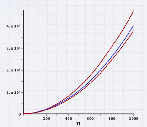
Suppose that we had two algorithms which sorted a list of size n and the runtime (in the number of instructions) is given by:

• \[b_{worst}(n)=4.7n^2-0.5n+5\]
• \[b_{best}(n)=3.8n^2+0.5n+5\]
• \[s(n)=4n^2+14n+12\]
• The smaller the value n, the fewer instructions are run
  • For \(n\leq 21\), \(b_{worst}(n)< s(n)\)
  • For \(n\geq 22\), \(b_{worst}(n)< s(n)\)
• With small values of n, the algorithm described by s(n) requires more instructions than even the \(b_{worst}(n)\)
  • Near n = 1000, \(b_{worst}(n)\approx 1.175 s(n)\) and \(b_{best}(n)\approx 0.95 s(n)\)

Is this a serious difference between these two algorithms?

• Because we can count the number instructions, we can also estimate how mush time is required to run one of these algorithms on a computer. Suppose that we have a 1GHz computer,
• The time (s) required to sort a list with 1 million elements, it will take about 1 second.
• If \(f(n)=a_{k}n^k+a_{k-1}n^{k-1}+...\) and \(g(n)=b_{k}n^k+b_{k-1}n^{k-1}+...\), \((a_{k}\neq 0, b_{k}\neq 0)\)
• For large enough n, it will always be true that \(f(n) < Mg(n)\) where, we choose \(M =\frac{a_k}{b_k} + 1\)
• In this case, we only need a computer which is M times faster.
• Unlike coefficient, the difference of polynomial cannot be covered by using a faster computer.

Weak Ordering

Consider the following definitions: We will consider two functions to be equivalent, \(f\sim g\), if \(\lim_{n \rightarrow \infty}\frac{f(n)}{g(n)}=c\) where, \(0 < c <\infty\) We will state that \(f<g\) if \(\lim_{n \rightarrow \infty}\frac{f(n)}{g(n)}=0\)

• These define a weak ordering
• Place \(n\) and \(n^2\) in the same line
• Let \(f(n)\) and \(g(n)\) describe either the run-time of two algorithms
• If \(f(n)\sim g(n)\), then it is always possible to improve the performance of one function over the other by purchasing a faster computer
• If \(f(n) < g(n)\), then you can never purchase a computer fast enough so that the second function always runs in less time than the first
  • In other words, you can firmly say f(n) is more efficient than g(n)

source “K-MOOC 허재필 교수님의 <인공지능을 위한 알고리즘과 자료구조: 이론, 코딩, 그리고 컴퓨팅 사고> 강좌의 5-1 함수의 점근적 분석법 중(http://www.kmooc.kr/courses/course-v1:SKKUk+SKKU_46+2020_T1)”

back next

Comments

Post comment

Loading...